Basic Example

Walkthrough

This section walks through a basic example of how to use OptoBot to implement an automated experimental optimisation loop for a colorimetric experiment. In this example, the experiment is mixing red, yellow and blue (RYB) food colouring along with water to produce a pre-defined target colour. One thing to note is that the water acts as a dilution agent and will not be included as a parameter in the search space for the optimisation algorithm. Instead, the volume of water is calculated as the remaining volume in a well after the red, yellow and blue food colouring volumes have been calculated. The experimental setup is shown below.

Figure: An example experimental setup for a colorimetric experiment.

We start with importing the required classes and functions from the optobot package. The first import includes the optobot.automate.OptimisationLoop class which implements the main automated experimental optimisation loop. The second import includes the optobot.colorimetric.get_colours function which handles capturing an image of the OT-2’s deck using a camera and retrieving the RGB values of wells in the image.

from optobot.automate import OptimisationLoop
from optobot.colorimetric.colours import get_colours

Next, we define the experimental setup and configuration. This starts with setting the experimental parameters and experimental response variables. For optimisation, the target experimental response, the experimental parameter search space and a relative tolerance are defined. The relative tolerance is set so that the optimisation loop stops if a measured experimental response is close enough to the target experimental response. Note that the target experimental response can be set to None if minimisation/maximisation based optimisation is desired instead of target based optimisation. However, the user should take into account that a target experimental response has not been set when defining their objective function. Also note that the dilution agent should be entered as the first experimental parameter because the first element will not be considered as part of the search space for optimisation.

# Define an experiment name.
experiment_name = "colour_experiment"

# Define the experimental parameters.
# In this experiment, these are RYB colour pigments and water.
# NOTE: The dilution agent should be entered as the first parameter.
liquid_names = ["water", "red", "yellow", "blue"]

# Define the measured parameters.
# In this experiment, these are the RGB values of the experimental products.
measured_parameter_names = ["measured_red", "measured_green", "measured_blue"]

# Set a target measurement.
# In this experiment, this a set of defined RGB values.
# NOTE: The target can be set to None for minimisation/maximisation based optimisation.
target_measurement = [
    114.8412698,
    96.1111111,
    37.84126984,
]  # Taken from a previous experiment.

# Set a relative tolerance (percentage).
# If a measurement is within the tolerance from the target, the optimisation loop is stopped.
relative_tolerance = 0.05

# Define the search space of the experimental parameters.
# In this experiment, this is the range of volumes for RYB colour pigments.
search_space = [[0.0, 30.0], [0.0, 30.0], [0.0, 30.0]]

Next, we define the well plate configuration inside the Opentrons OT-2. This includes well plate dimensions and well plate location on the OT-2’s deck. Note that multiple well plates can be used through defining a list of well plate locations. If multiple well plate locations are defined, each well plate is used in a sequential manner. We also define the maximum liquid volume of each well.

# Define the well plate dimensions.
wellplate_size = 96
wellplate_shape = (8, 12)  # As (rows, columns).

# Define the total volume in a well.
total_volume = 90.0

# Define the location of the wellplate in the Opentrons OT-2.
# In this experiment, this is slot 5.
# NOTE: More than one well plate can be used.
# NOTE: For example, slots 5 & 8 -> [5, 8]
wellplate_locs = [5]

Next, we define the population size and the number of iterations for the optimisation algorithm. Note that we should make sure that the combination of population size and number of iterations do not exceed the total number of available wells.

# Define the population size for optimisation.
# In this experiment, this is defined as 12 -> 12 wells/columns.
population_size = 12

# Define the number of iterations for optimisation.
# In this experiment, this is defined as 8 -> 8 rows.
num_iterations = 8

# Check that the number of iterations and population size are valid.
if population_size * num_iterations > wellplate_size * len(wellplate_locs):
    print("error: not enough wells for defined population and iteration size")
    sys.exit(1)

Next, we define an objective function for experimental optimisation. In this example, we use the squared Euclidean distance between the target RGB values and the measured RGB values as the objective function.

\[{||x - y||}^{2} = \sum_{i} (x_{i} - y_{i})^{2}\]

# Define an objective function for optimisation.
def objective_function(measurements):
    """
    The objective function to be optimised.

    In this experiment, this calculates the squared Euclidean distance
    between the target RGB value and the measured RGB values.

    Parameters
    ----------
    measurements : np.ndarray
        The measured parameter values of the experimental products.

    Returns
    -------
    errors : np.ndarray
        The errors between the target value and the measured values.
    """

    errors = ((measurements - target_measurement) ** 2).sum(axis=1)
    return errors

Next, we define a measurement function for measuring the experimental products between each iteration of optimisation. As this example is a colorimetric experiment, we can utilise the optobot.colorimetric.get_colours function to handle the entire process of capturing an image of the OT-2’s deck and retrieving the RGB values of the experimental products. Note that a measurement function does not have to be defined if a manual measurement process is used between iterations of optimisation. However, a manual measurement process will require manual inputs of the measured experimental response variables. A custom measurement function that interfaces with other equipment can also be used instead of the get_colours function to measure different experimental response variables.

# Define a measurement function for measuring experimental products.
# NOTE: A measurement function does not have to be defined if measurement input is manual.
def measurement_function(
    liquid_volumes,
    iteration_count,
    population_size,
    num_measured_parameters,
    data_dir,
):
    """
    The measurement function for measuring experimental products.

    In this experiment, this uses the "get_colours" function from the
    "optobot.colorimetric.colours" sub-module. The "get_colours" function
    uses a webcam pointing at the OT-2 deck to take a picture and retrieve
    the RGB values of the experimental products.

    Parameters
    ----------
    liquid_volumes : np.ndarray
        The liquid volumes of the experimental parameters used to generate
        the experimental products in the current iteration.

    iteration_count : int
        The current iteration.

    population_size : int
        The population size.

    num_measured_parameters : int
        The number of measured parameters.

    data_dir : string
        The directory for storing the experimental data.

    Returns
    -------
    np.ndarray, float[population_size, num_measured_parameters]
        The measured parameter values of the experimental products.
    """

    return get_colours(
        iteration_count, population_size, num_measured_parameters, data_dir
    )

To finalise, we initialise an instance of the optobot.automate.OptimisationLoop class with the variables and functions we have defined. We then call the OptimisationLoop.optimise class method to begin the automated optimisation loop. Note that we use Particle Swarm Optimisation in this example, but Bayesian Optimisation can also be used through setting the optimiser parameter to “GP” for Gaussian Process as the acquisition function or “RF” for Random Forest as the acquisition function.

# Define the automated optimisation loop.
model = OptimisationLoop(
    objective_function=objective_function,
    liquid_names=liquid_names,
    measured_parameter_names=measured_parameter_names,
    target_measurement = target_measurement,
    population_size=population_size,
    name=experiment_name,
    measurement_function=measurement_function,
    wellplate_shape=wellplate_shape,
    wellplate_locs=wellplate_locs,
    total_volume=total_volume,
    relative_tolerance= relative_tolerance,
)
# Start the optimisation loop.
# In this experiment, Particle Swarm Optimisation is used.
model.optimise(search_space, optimiser="PSO", num_iterations=num_iterations)

Once the optimisation loop has started, an OT-2 protocol script will be generated with the first set of experimental parameter values and the following text will be outputted to the command line. The user should upload and run the OT-2 protocol script using the Opentrons App.

2025-04-06 22:00:00,000 - pyswarms.single.global_best - INFO - Optimize for 8 iters with {'c1': 0.3, 'c2': 0.5, 'w': 0.1}
pyswarms.single.global_best:   0%|                                                                                        |0/8
Upload script, wait for robot, and then press any key to continue:

After the OT-2 is finished with the protocol, the user should continue the program which will result in the measurement function being called. In this example, this is the get_colours function which will first capture an image of the OT-2’s deck. A prompt for a threshold parameter, which controls how sensitive the contour detection algorithm should be, will then appear on the command line. A higher threshold will make the contour detection algorithm more sensitive and vice versa. The contour detection algorithm will then attempt to locate the wells in the image of the OT-2’s deck and the user will be prompted to either accept the results or redo the contour detection algorithm. The user can also decide to use a manual extrapolated grid algorithm instead of the contour detection algorithm to locate the wells in the image. To use the manual extrapolated grid algorithm, the user will be prompted to click on two consecutive wells in the image from which an extrapolated grid of well locations is calculated. This process can be repeated until the wells in the image are located to the user’s desired precision.

Type threshold (Default is 30):
30

Happy with detection?
type "y" if you are, "n" to try again, and "b" to use the manual clicking detection
b
Happy with the grid? [y/n] y

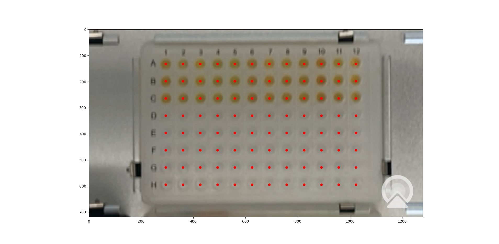
Figure: An example image of located wells using the extrapolated grid algorithm.

Once an image with located wells has been accepted, the RGB values of the experimental products from the current iteration of optimisation will be fed to the optimisation algorithm. If the target experimental response has not been achieved, the optimisation algorithm will generate a new OT-2 protocol script with the next experimental parameter values and the following text will be outputted to the command line. The process described in the above paragraphs is then repeated until either the target experimental response is achieved or the defined number of optimisation iterations are completed.

pyswarms.single.global_best:  12%|██████████████████                                                                        |1/8, best_cost=17362.0
Upload script, wait for robot, and then press any key to continue:

If a measured experimental response falls within the defined tolerance from the target experimental response, the target experimental response is considered to be achieved. The optimisation process is stopped and the following text will be outputted to the command line.

pyswarms.single.global_best:  75%|█████████████████████████████████████████████████████████████████████████████████████            |6/8, best_cost=1.08
Upload script, wait for robot, and then press any key to continue:

Stopping the optimization - measurements have been found that are close to the target (within 5.0%):
- measurement = [14.43234437 20.13919216 14.3225938 ], percent differences of each value to the target values = [3.09 0.7  4.52]%

Note: All measured and generated data is saved to a folder with the experiment name.

Full Script

The full script for the example is given below.

"""
An example script showing how to use the optobot package. This script uses the
optobot package in the context of a colour mixing experiment, where red, yellow
and blue (RYB) liquid pigments are mixed to create a target colour.
"""

# Import required libraries.
import sys

from optobot.automate import OptimisationLoop
from optobot.colorimetric.colours import get_colours


def main():
    # Define an experiment name.
    experiment_name = "colour_experiment"

    # Define the experimental parameters.
    # In this experiment, these are RYB colour pigments and water.
    # NOTE: The dilution agent should be entered as the first parameter.
    liquid_names = ["water", "red", "yellow", "blue"]

    # Define the measured parameters.
    # In this experiment, these are the RGB values of the experimental products.
    measured_parameter_names = ["measured_red", "measured_green", "measured_blue"]

    # Set a target measurement.
    # In this experiment, this a set of defined RGB values.
    # NOTE: The target can be set to None for minimisation/maximisation based optimisation.
    target_measurement = [
        114.8412698,
        96.1111111,
        37.84126984,
    ]  # Taken from a previous experiment.

    # Set a relative tolerance (percentage).
    # If a measurement is within the tolerance from the target, the optimisation loop is stopped.
    relative_tolerance = 0.05

    # Define the search space of the experimental parameters.
    # In this experiment, this is the range of volumes for RYB colour pigments.
    search_space = [[0.0, 30.0], [0.0, 30.0], [0.0, 30.0]]

    # Define the well plate dimensions.
    wellplate_size = 96
    wellplate_shape = (8, 12)  # As (rows, columns).

    # Define the total volume in a well.
    total_volume = 90.0

    # Define the location of the wellplate in the Opentrons OT-2.
    # In this experiment, this is slot 5.
    # NOTE: More than one well plate can be used.
    # NOTE: For example, slots 5 & 8 -> [5, 8]
    wellplate_locs = [5]

    # Define the population size for optimisation.
    # In this experiment, this is defined as 12 -> 12 wells/columns.
    population_size = 12

    # Define the number of iterations for optimisation.
    # In this experiment, this is defined as 8 -> 8 rows.
    num_iterations = 8

    # Check that the number of iterations and population size are valid.
    if population_size * num_iterations > wellplate_size * len(wellplate_locs):
        print("error: not enough wells for defined population and iteration size")
        sys.exit(1)

    # Define an objective function for optimisation.
    def objective_function(measurements):
        """
        The objective function to be optimised.

        In this experiment, this calculates the squared Euclidean distance
        between the target RGB value and the measured RGB values.

        Parameters
        ----------
        measurements : np.ndarray
            The measured parameter values of the experimental products.

        Returns
        -------
        errors : np.ndarray
            The errors between the target value and the measured values.
        """

        errors = ((measurements - target_measurement) ** 2).sum(axis=1)
        return errors

    # Define a measurement function for measuring experimental products.
    # NOTE: A measurement function does not have to be defined if measurement input is manual.
    def measurement_function(
        liquid_volumes,
        iteration_count,
        population_size,
        num_measured_parameters,
        data_dir,
    ):
        """
        The measurement function for measuring experimental products.

        In this experiment, this uses the "get_colours" function from the
        "optobot.colorimetric.colours" sub-module. The "get_colours" function
        uses a webcam pointing at the OT-2 deck to take a picture and retrieve
        the RGB values of the experimental products.

        Parameters
        ----------
        liquid_volumes : np.ndarray
            The liquid volumes of the experimental parameters used to generate
            the experimental products in the current iteration.

        iteration_count : int
            The current iteration.

        population_size : int
            The population size.

        num_measured_parameters : int
            The number of measured parameters.

        data_dir : string
            The directory for storing the experimental data.

        Returns
        -------
        np.ndarray, float[population_size, num_measured_parameters]
            The measured parameter values of the experimental products.
        """

        return get_colours(
            iteration_count, population_size, num_measured_parameters, data_dir
        )

    # Define the automated optimisation loop.
    model = OptimisationLoop(
        objective_function=objective_function,
        liquid_names=liquid_names,
        measured_parameter_names=measured_parameter_names,
        target_measurement=target_measurement,
        relative_tolerance=relative_tolerance,
        population_size=population_size,
        name=experiment_name,
        measurement_function=measurement_function,
        wellplate_shape=wellplate_shape,
        wellplate_locs=wellplate_locs,
        total_volume=total_volume
    )

    # Start the optimisation loop.
    # In this experiment, Particle Swarm Optimisation is used.
    model.optimise(search_space, optimiser="PSO", num_iterations=num_iterations)


if __name__ == "__main__":
    main()